Mean-field homogenization of polycrystals: estimating effective elastic properties
Metals are composed of anisotropic grains that develop preferred orientations (textures) during processing, leading to anisotropy in their macroscopic properties. This article explores mean-field homogenization methods for estimating effective elastic properties and presents an open-source MATLAB script for analyzing anisotropy in deformation textures.
This page is still under development.
1 Introduction
In polycrystalline materials, the effective elastic properties are governed by both the intrinsic elastic constants of the individual grains (single crystals) and the way in which these grains are oriented. When the grains are randomly oriented, the effective behaviour of a polycrystal can be approximated as isotropic. However, in many practical situations, grains exhibit a preferential orientation—known as texture—which introduces anisotropy into the material’s overall behavior. Metallic materials develop textures primarily due to the processing methods they undergo. During deformation processes such as rolling, forging, extrusion, or drawing, the grains in the metal reorient themselves to accommodate the applied stresses. This reorientation is driven by the activation of specific slip systems in the crystal lattice, resulting in a non-random, preferred orientation of grains. Additionally, subsequent thermal treatments like annealing can lead to recrystallization, where new grains form with orientations influenced by the deformed structure, further reinforcing the texture. In essence, the combination of mechanical deformation and thermal processing causes metallic materials to develop textures that significantly influence their macroscopic properties. Ideally, to fully capture the influence of textures on effective properties, one would need detailed information on both the orientation distribution and the shape and size distributions of the grains. In reality, this comprehensive data is difficult to obtain and incorporate due to the complexity and computational demands of the calculations. Consequently, it is common practice to assume that only the grain orientation influences the effective elastic constants, while the variations in grain shape and spatial arrangement are neglected.
In the following, a brief introduction to elastic anisotropy, crystallographic texture and, its representation is discussed. In section 2, the most common methods (The Voigt-Reuss-Hill approach and the self-consistent method) to calculate the effective elastic properties of polycrystals are discussed. In section 3, the developed MATLAB code is validated by considering extreme cases and in section 4, the anisotropy of effective elastic tensor for deformation textures is discussed.
1.1 Elastic anisotropy
Single crystals of metallic materials are periodic in nature which makes them inherently anisotropic. The Figure 1 shows the variation of Young’s modulus with the crystallographic direction in an Fe single crystal. Compared to the generally assumed isotropic value (210 GPa), the value fluctuates with the crystallographic direction.
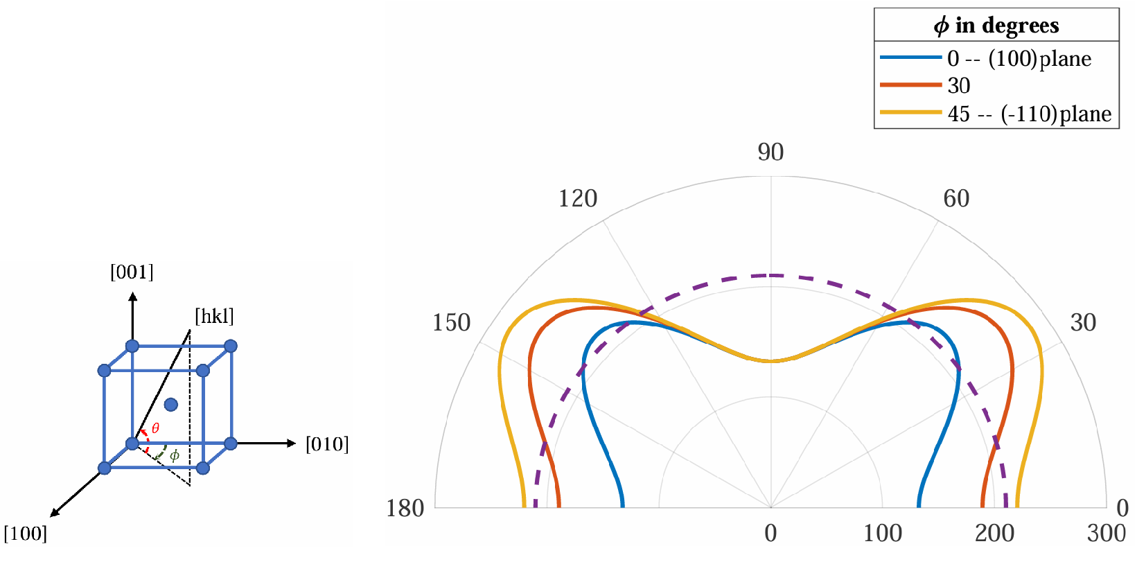 Figure 1: The variation of Young’s modulus with the crystallographic direction in Fe single crystal ($\theta$ = 0 to 180 degrees)
The generalized Hooke’s law for fully anisotropic linear elastic materials is
\[\sigma_{ij} = C_{ijkl} \varepsilon^\mathrm{e}_{kl},\]where $C_{ijkl}$ is a fourth-order stiffness tensor consisting of 81 material constants. Due to its major and minor symmetries, the number of required material constants reduces to 21. And Hooke’s law is represented in Voigt notation as
\[\boldsymbol\sigma = \mathbf C\ {\boldsymbol\varepsilon}^{\mathrm{e}} \equiv \begin{bmatrix} \sigma_1 \\ \sigma_2 \\ \sigma_3 \\ \tau_4 \\ \tau_5 \\ \tau_6 \end{bmatrix}= \begin{bmatrix} C_{11} & C_{12} & C_{13} & C_{14} & C_{15} & C_{16} \\ & C_{22} & C_{23} & C_{24} & C_{25} & C_{26} \\ & & C_{33} & C_{34} & C_{35} & C_{36} \\ & & & C_{44} & C_{45} & C_{46} \\ & \text{sym} & & & C_{55} & C_{56} \\ & & & & & C_{66} \\ \end{bmatrix} \begin{bmatrix} {\varepsilon^{\mathrm{e}}}_1 \\ {\varepsilon^{\mathrm{e}}}_2 \\ {\varepsilon^{\mathrm{e}}}_3 \\ {\gamma^{\mathrm{e}}}_4 \\ {\gamma^{\mathrm{e}}}_5 \\ {\gamma^{\mathrm{e}}}_6 \end{bmatrix},\]where the elastic stiffness matrix $\textbf C$ of a material is described by a $6\times6$ symmetric matrix.
The number of required material constants will further reduce due to material symmetries. For the fully anisotropic triclinic structure, 21 material constants are required. For monoclinic - 13, orthorhombic - 9, tetragonal - 6 and hexagonal - 5 material constants are required. For cubic materials, only three material constants viz. $C_{11}$, $C_{12}$ and $C_{44}$ are required. i.e.,
\[\mathbf{C} = \begin{bmatrix} C_{11} & C_{12} & C_{12} & 0 & 0 & 0 \\ & C_{11} & C_{12} & 0 & 0 & 0 \\ & & C_{11} & 0 & 0 & 0 \\ & & & C_{44} & 0 & 0 \\ & \text{sym} & & & C_{44} & 0 \\ & & & & & C_{44} \end{bmatrix}\ .\]For isotropic materials, the no of material constants reduces to 2 viz. $C_{11}$, $C_{12}$ or Young’s modulus ($E$) and Poisson’s ratio ($\nu$).
1.2 Crystallographic textures
All crystalline materials, most of the time, are polycrystals and made of many grains with different orientations. It is very rare that these orientations are completely random. A pattern in the orientation distribution will develop during solidification or by the mechanical processing route. Such a preferred orientation is called ‘texture’. The presence of texture in a material causes anisotropy and affects the overall material properties, such as Young’s modulus, ductility, strength, Poisson’s ratio and magnetic permeability.
The crystallographic orientation is generally represented by
- Miller indices
- Orientation matrix ($\mathbf Q$)
- Euler angles
- Miller Indices
- This representation is mostly used for rolled sheet materials and represented as a combination of the rolling plane (ND) $\lbrace\mathrm{hkl}\rbrace$ and Rolling Direction (RD) $\langle\mathrm{uvw}\rangle$ shown in the Figure 2. This is interpreted as the $\lbrace\mathrm{hkl}\rbrace$ planes of the majority of the grains are parallel to the rolling plane of the sheet, and the crystallographic direction $\langle\mathrm{uvw}\rangle$ of these grains is in the direction of RD of the sheet.
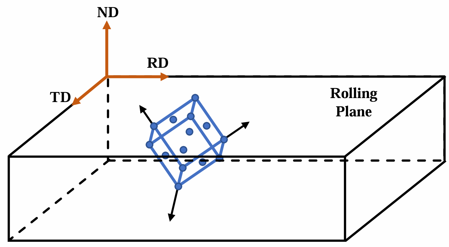 Figure 2: Rolled sheet material
- Orientation Matrix ($\mathbf Q$)
- The orientation matrix is a transformation matrix that transforms a vector from Sample Coordinate System (SCS) to Crystal Coordinate System (CCS). Let $\mathbf a_c$ and $\mathbf a_s$ be the vectors in CCS and SCS, respectively.
- Euler Angles ($\phi_1, \Phi,\phi_2$)
- Euler angles are the three sequential rotations required to describe a transformation from the SCS ($XYZ$) to the CCS ($\langle 1\ 0\ 0\rangle$). Several conventions are available to express Euler angles. Bunge’s notation is the one most commonly used. According to Bunge’s notation (Figure 4),
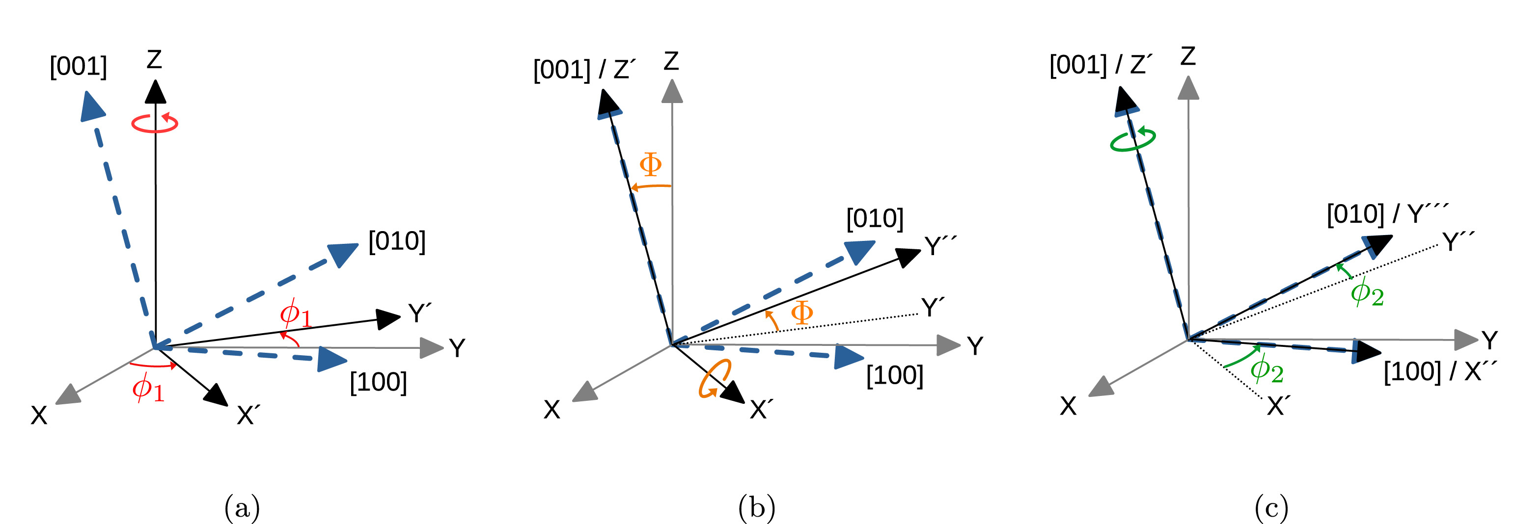 Figure 4: Representation of Euler angles as defined by Bunge notation: (a) rotation by $\phi_1$, (b) rotation by $\Phi$, and (c) rotation by $\phi_2$1
- A rotation by $\phi_1$ about the $Z-$axis, transforming the $Y-$axis to $Y’$ and the $X-$axis to $X’$.
- A rotation by $\Phi$ about the $X’-$axis, transforming the $Z-$axis to $Z’$ i.e., $[0\ 0\ 1]$ and the $Y’-$axis to $Y’’$.
- A rotation by $\phi_2$ about the $Z’-$axis, transforming the $Y’’-$axis to $Y’’’$ i.e., $[0\ 1\ 0]$ and the $X’-$axis to $X’’$ i.e., $[1\ 0\ 0]$.
Where $\phi_1$,$\Phi$ and $\phi_2$ are the Euler angles. The elements of the ‘$\mathbf{Q}$’ matrix can be expressed as a function of Euler angles as follows:
\[\begin{equation}\label{eq:orimateuler} \begin{aligned} g_{11} &= \cos\phi_1 \cos\phi_2 - \sin\phi_1\sin\phi_2\cos\Phi \\ g_{12} &= \sin\phi_1\cos\phi_2 + \cos\phi_1\sin\phi_2\cos\Phi \\ g_{13} &= \sin\phi_2\sin\Phi \\ g_{21} &= -\cos\phi_1\sin\phi_2 - \sin\phi_1\cos\phi_2\cos\Phi \\ g_{22} &= - \sin\phi_1\sin\phi_2 + \cos\phi_1 \cos\phi_2\cos\Phi \\ g_{23} &= \cos\phi_2\sin\Phi \\ g_{31} &= \sin\phi_1\sin\Phi \\ g_{32} &= - \cos\phi_1\sin\Phi \\ g_{33} &= \cos\Phi \ . \end{aligned} \end{equation}\]2 Mean-field approaches for estimating effective elastic properties
In the following sections, different mean field methods to calculate the effective elastic constants of polycrystals are discussed. The Voigt-Reuss-Hill methods assume uniform stress or uniform strain throughout the polycrystal. Whereas the self-consistent approach proposed by Kroner derives an effective stress-strain relation using the Eshelby solution. The elastic constants of a single crystal are material properties and usually can be obtained from experiments. However, they are described in the crystal reference frame. In the following methods, these constants are calculated in the sample reference frame with the help of the orientation information, often expressed in Euler angles.
\[\mathbb{C}^s_{ijkl} = \mathbf{Q}^\mathrm{T}_{ii'}\mathbf{Q}^\mathrm{T}_{jj'}\mathbf{Q}^\mathrm{T}_{kk'}\mathbf{Q}^\mathrm{T}_{ll'}\mathbb{C}^c_{i'j'k'l'}\]Note: In this context, the grains are assumed to have equal size and shape. Hence, the volume fractions are constant.
2.1 Voigt approximation
The Voigt approximation is derived from the assumption that the total strain is uniform within the polycrystal. This ensures strain compatibility throughout the polycrystal but not necessarily the stress equilibrium. The averaged elastic constants follow from the weighted average of stiffness tensor over all orientations of the grains present within the polycrystal. The Voigt approximation gives too-large values for the effective elastic constants; hence, It is considered as the upper bound for the stiffness tensor.
\[\mathbb{C}^V = \left\langle \mathbb{C}^c \right\rangle\]where $\mathbb{C}^c$ is the stiffness tensor of a single crystal in the sample reference frame.
2.2 Reuss approximation
The Reuss approximation is derived from the assumption that the total stress is uniform within the polycrystal. This ensures the stress equilibrium throughout the polycrystal but not necessarily the strain compatibility. The averaged elastic constants follow from the weighted average of the compliance tensor over all orientations of the grains present within the polycrystal. The Reuss approximation gives the upper bound for the compliance tensor, hence the lower bound for the stiffness tensor.
\[\mathbb{C}^R = \left\langle \mathbb{C}^{c^{-1}} \right\rangle^{-1}\]where $\mathbb{C}^c$ is the stiffness tensor of a single crystal in the sample reference frame.
2.3 Hill approximation
In general, The Voigt and Reuss bounds fall not too far from the actual values. Hence, Hill suggested using the arithmetic mean of the Voigt and Reuss bounds as a reasonable empirical estimate of the overall moduli.
\[\mathbb{C}^H = \frac{1}{2}\left[ \left\langle \mathbb{C}^c \right\rangle + \left\langle \mathbb{C}^{c^{-1}} \right\rangle^{-1}\right]\]where $\mathbb{C}^c$ is the stiffness tensor of a single crystal in the sample reference frame.
Even though the deviation of the Hill approximation from actual values is nearly independent of the texture of the polycrystal, it fails in the case of large grain shape anisotropy. But it is quite useful to describe texture dependence of the elastic properties and also serves as the initial guess for the more accurate self-consistent method, which is implicit in nature.
2.4 Self-consistent method
The problem of finding the stress induced in the inclusion by a remotely applied stress (at an infinite distance) is referred to as Eshelby’s problem. The solution to this problem was first obtained by Eshelby in terms of elastic Green’s function. A self-consistent method that makes use of this result was first proposed by Kroner, who assumed that the grains could be regarded as inclusions embedded in a Homogenous Effective Medium(HEM) having the average elastic properties of the aggregate. From the average stress theorem, the expression for the effective stiffness tensor is
\[\begin{equation}\label{eq:selfconsit} \mathbb{C} = \langle \mathbb{C}^c\mathbb{A} \rangle, \quad \mathbb{A} = \left[\mathbb{I}+\mathbb{S}\mathbb{C}^{-1}\left(\mathbb{C}^c-\mathbb{C}\right)\right]^{-1} \end{equation}\]where $\mathbb{C}^c$ is the stiffness tensor of a single crystal in the sample reference frame, $\mathbb{A}$ is the strain concentration tensor, and $\mathbb{S}$ is the Eshelby tensor.
It can be seen that the above equation is implicit in nature. Hence, requires solving iteratively. The Hill approximation serves as a good initial guess for the iterative approach. The Eshelby tensor $\mathbb{S}$ is a function of the effective elastic constants of the HEM and the aspect ratios of the ellipsoid inclusion. The expressions to calculate the $\mathbb{S}$ following 2, are given below.
\[\mathbb{S}_{ijmn} = \frac{1}{4}\left(\Gamma_{ikjl}+\Gamma_{iljk}+\Gamma_{jkil}+\Gamma_{jlik}\right)\mathbb{C}_{klmn} = \Gamma^{sym}:\mathbb{C}\]where,
\[\Gamma_{ikjl} = \frac{1}{4\pi}\int_0^\pi\sin{\theta}d\theta\int_0^{2\pi}\gamma_{ikjl}d\phi,\] \[\gamma_{ikjl} = \text{K}^{-1}_{ik}\left(\xi\right)\xi_j\xi_l,\] \[\text K_{ip} = \mathbb{C}_{ijpl}\xi_j\xi_l,\] \[\text{and } \xi_1 = \frac{\sin\theta\cos\phi}{a_1}\quad;\quad \xi_2 = \frac{\sin\theta\sin\phi}{a_2}\quad;\quad \xi_3 = \frac{\cos\theta}{a_3}.\]Here $0<\phi<2\pi$ and $0<\theta<\pi$ are spherical coordinates that define the direction of the vector $\xi$ with respect to the principal axes of the ellipsoid of length $2a_1,2a_2,2a_3$. $\Gamma_{ikjl}$ is computed using the numerical integration technique of extended trapezoidal rule (refer Appendix) over the specified intervals with an increment of $2^o$ in each dimension
The Equation \ref{eq:selfconsit}, however, is valid only under the assumption that all the ellipsoids representing the grains have the same shape and orientation. Otherwise, both the expressions, one from the average stress theorem (Equation \ref{eq:selfconsit}) and one from the average strain theorem have to be solved simultaneously.
Note: In this context, the principal axes of the ellipsoid are assumed to coincide with the axis of the sample reference frame
3 Verification and validation of the MATLAB implementation
The anisotropy of a polycrystal is essentially affected by two factors: the single-crystal anisotropy and the texture. Based on this, the developed MATLAB code to calculate the effective elastic constants of a textured polycrystal is tested for the following four extreme cases:
- Random texture of anisotropic grains - isotropic aggregate
- Random texture of isotropic grains - isotropic aggregate
- Highly textured polycrystal of anisotropic grains - anisotropic aggregate
- Highly textured polycrystal of isotropic grains - isotropic aggregate
3.1 Random texture of anisotropic grains - isotropic aggregate
The effective stiffness tensor is calculated using the self-consistent method for the Copper ($C_{11}$ = 168 GPa, $C_{12}$ = 121.4 GPa, $C_{44}$ = 75.4 GPa) polycrystal with a completely random texture. Five different random textures were generated using the open-source MTEX toolbox 3 with the number of grains 1000, 10000, 20000, 30000 and 60000. The anisotropy of the stiffness tensor for these textures is studied in the following two ways
- Using Tensor Anisotropy Index
- With the help of eigenvalues
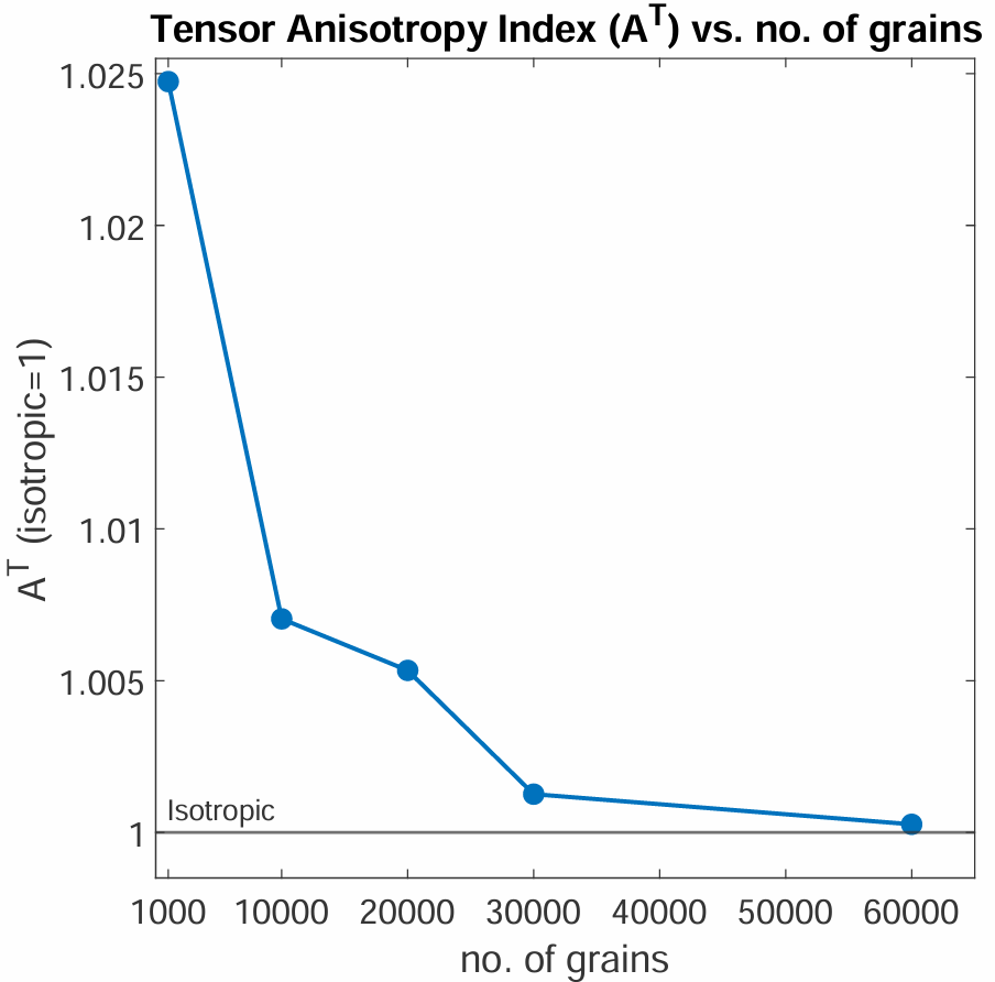 Figure 5: Tensor Anisotropy Index ($A^T$)
The Tensor Anisotropy Index($A^T$) 4 is a measure of anisotropy of stiffness tensor and is equal to 1 for an isotropic material. The formula for calculating $A^T$ is provided in the appendix. $A^T$ is calculated for all the effective stiffness tensors of different random textures and plotted in Figure 5. From the figure, it can be observed that with the increase in the number of orientations, the value of $A^T$ is decreasing and reaching the value ‘1’. The $A^T$ for an isotropic material is ‘1’; hence it can be stated that the polycrystal aggregate with random texture is isotropic in nature.
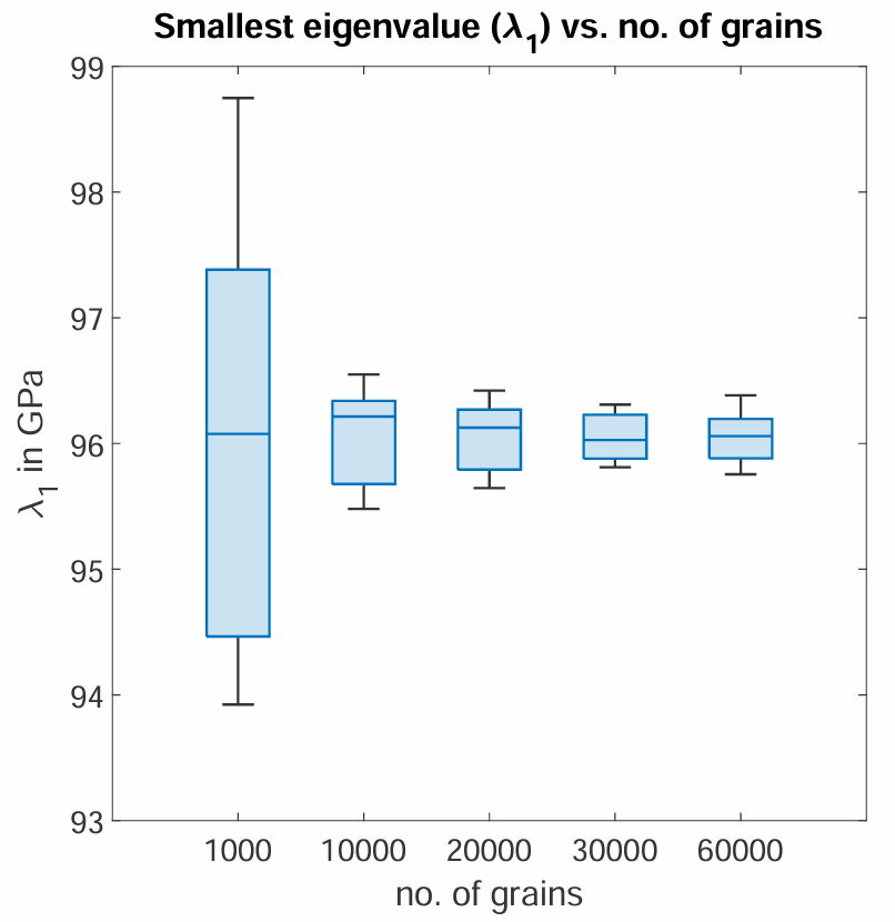 Figure 6: Smallest eigenvalue ($\lambda_1$)
Another way of verifying whether the effective stiffness tensor is isotropic is by calculating the eigenvalues of the tensor. For an isotropic material, 5 of the six eigenvalues of a stiffness tensor are equal. These eigenvalues are calculated for different random textures, and the data is visualized using boxplot as shown in Figure 6. From the figure, it can be seen that the range of the eigenvalues is decreasing with an increase in the no of orientations and reaching a mean value of 96.06 GPa. The eigenvalues for the upper bound, a lower bound and self-consistent estimate of a random texture with 60000 orientations are tabulated in Table 1.
Table 1: Eigenvalues of effective stiffness tensor (60000 orientations)
| Eigenvalues | 1 | 2 | 3 | 4 | 5 | 6 |
|---|---|---|---|---|---|---|
| Voigt | 410.8000 | 109.4392 | 109.2006 | 109.1276 | 108.9977 | 108.8349 |
| Reuss | 410.8000 | 79.8910 | 79.6749 | 79.6091 | 79.4920 | 79.3459 |
| Self-consistent | 410.8000 | 94.6651 | 94.4378 | 94.3683 | 94.2449 | 94.0904 |
Study of anisotropy in random texture
The directional Young’s modulus gives a proper description of elastic anisotropy. For all the random textures, the directional Young’s modulus is plotted using a spherical plot (Figure 7). From the figure, a steady decrease in the amount of anisotropy can be observed with an increase in the number of orientations, and Young’s modulus approaches the value of 129 GPa.
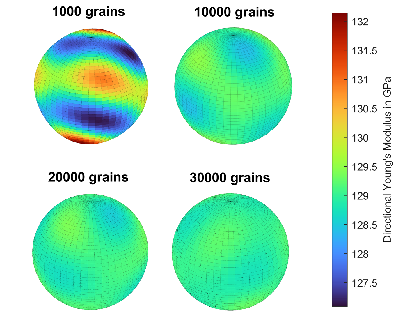 Figure 7: Directional Young’s modulus plotted for random textures with increasing no. of orientations
In cases 2 and 4, The estimated effective stiffness tensor is isotropic and agrees with both the Voigt and Reuss bounds. In case 3, a texture of completely cube orientation is taken, and the estimated effective stiffness tensor is equal to the stiffness tensor of the single crystal, which is to be expected.
3.2 Random texture of isotropic grains - isotropic aggregate
3.3 Highly textured polycrystal of anisotropic grains - anisotropic aggregate
3.4 Highly textured polycrystal of isotropic grains - isotropic aggregate
4 Estimation of elastic anisotropy in textured polycrystals
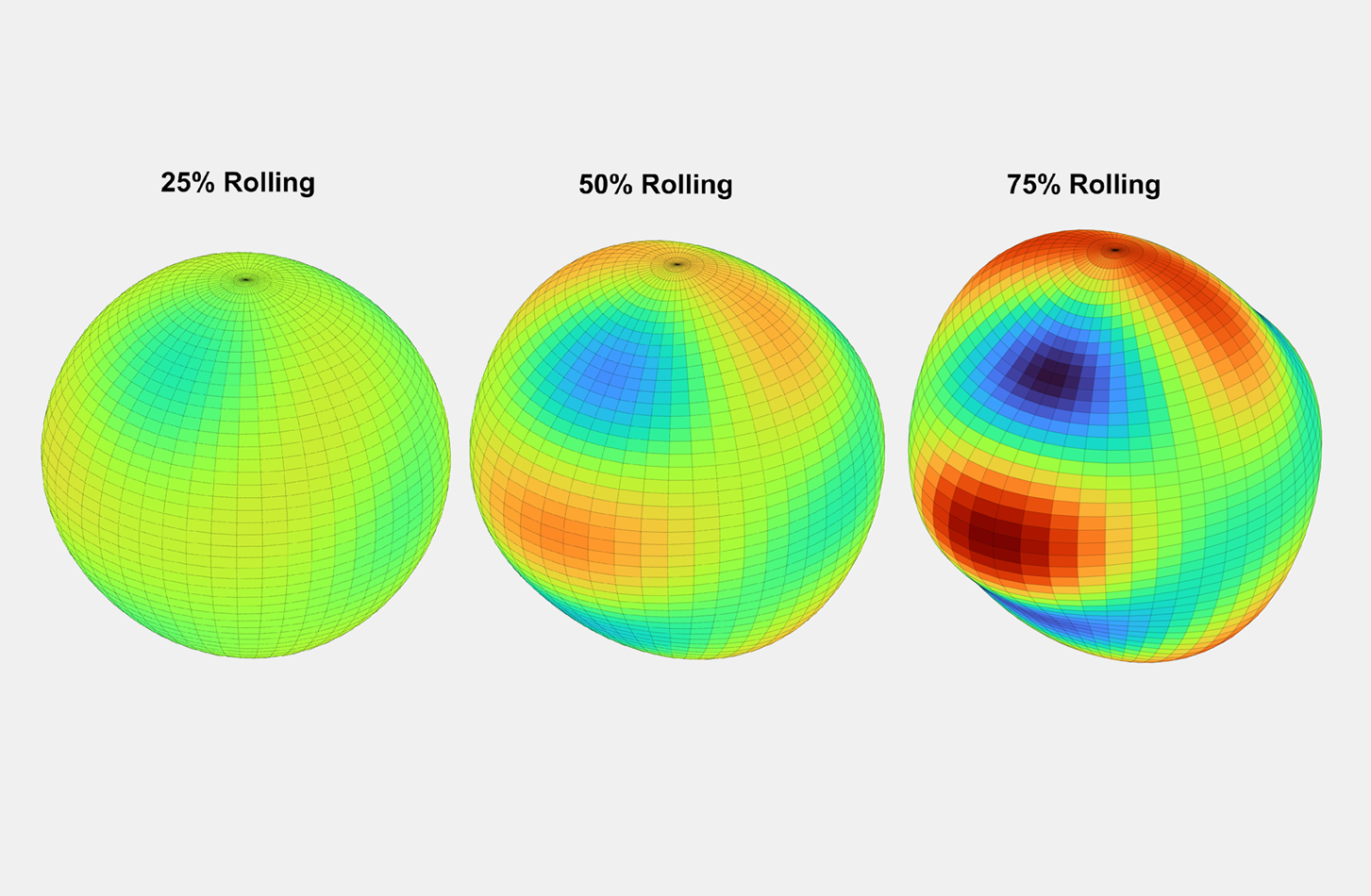
In this section, the directional variation of Young’s modulus is presented for different deformation textures, viz. rolling, uniaxial tension and shear deformation for both BCC(Fe) and FCC(Cu) materials. For both materials, an initial random texture of 1000 orientation is taken, and textures are obtained at a strain of 25%, 50% and 75% from the Taylor model. The obtained textures are used to calculate effective stiffness tensors using the self-consistent method, and the directional Young’s modulus is visualized using spherical plots. In case of rolling, the effect of grain shape on elastic properties is also presented by considering equiaxial and pancake shaped grains. In the rolling process, grains are usually elongated and flat. To represent the shape of the grain (at least to some extent), an ellipsoid with an aspect ratio of 5:1:0.2 for the rolling, transverse and normal directions respectively, is taken.
4.1 BCC textures
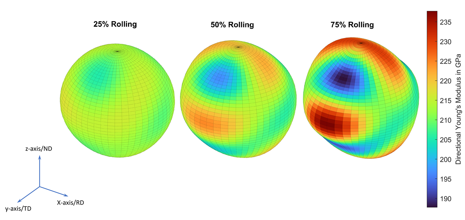 Figure 8: Evolution of elastic anisotropy in BCC materials during rolling.
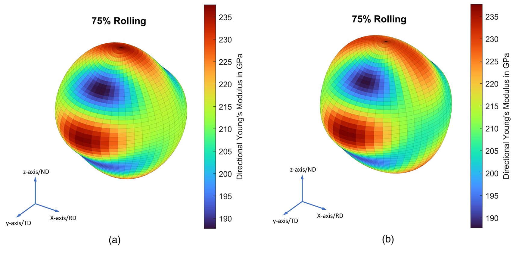 Figure 9: Effect of grain shape in rolling textures of BCC materials: (a) Rolling: spherical shape (1:1:1), (b) Rolling: pancake shape (5:1:0.2)
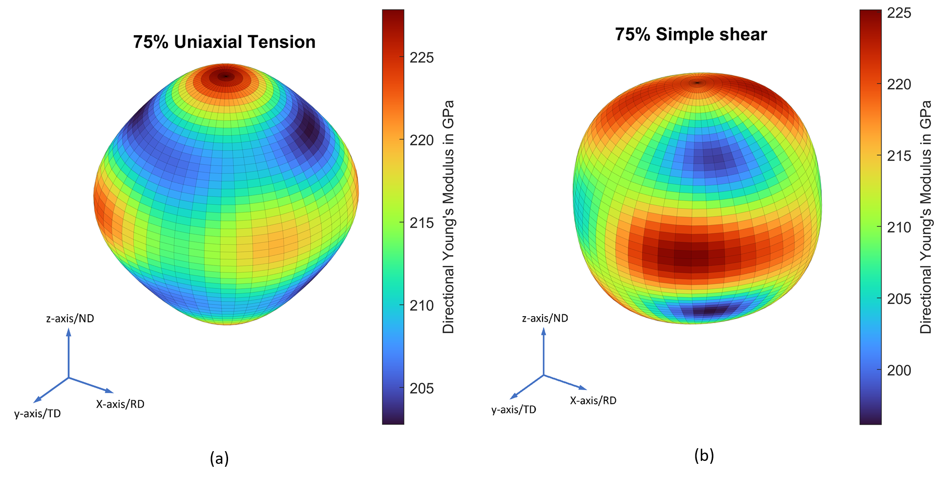 Figure 9: Deformation textures of BCC materials: (a) Uniaxial tension along $Z$-axis/ND, (b) Simple shear in $YZ$-plane along $X$-axis/RD
4.2 FCC textures
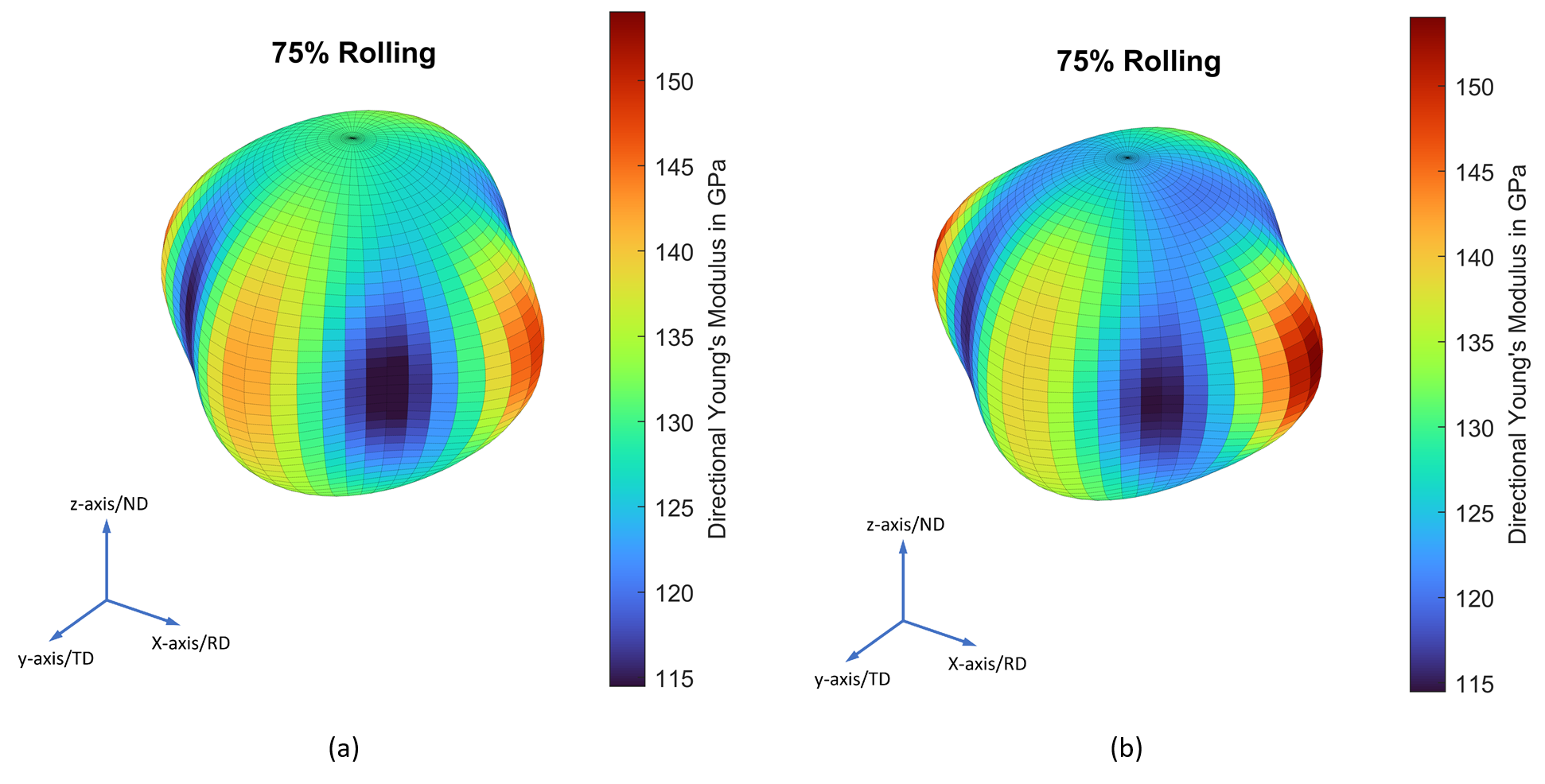 Figure 9: Effect of grain shape in rolling textures of FCC materials: (a) Rolling: spherical shape (1:1:1), (b) Rolling: pancake shape (5:1:0.2)
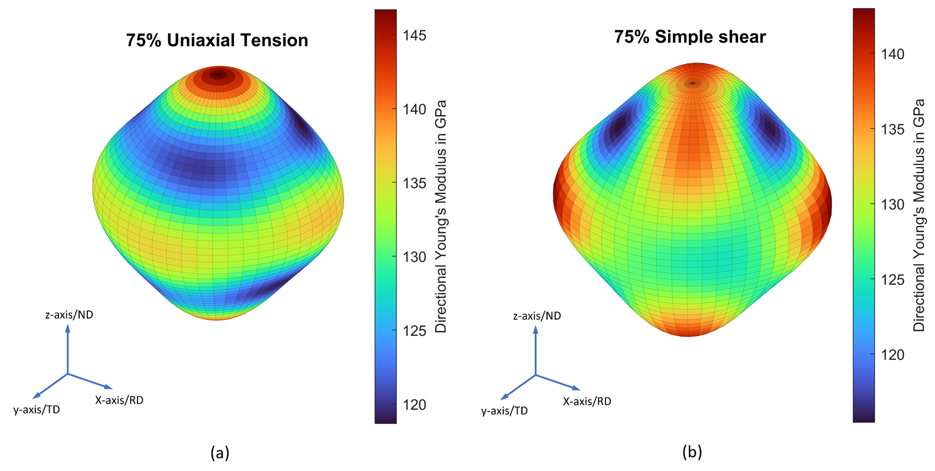 Figure 9: Deformation textures of FCC materials: (a) Uniaxial tension along $Z$-axis/ND, (b) Simple shear in $YZ$-plane along $X$-axis/RD
5 Conclusion
In this study, we explored the origins of elastic anisotropy in polycrystals, which arise from the inherent anisotropy of single crystals and the preferred orientation of grains due to processing-induced texture. To compute the effective elastic properties of a polycrystal, information on the orientation and shape distribution of grains is essential. We reviewed different mean-field approaches, including the Voigt-Reuss-Hill method and the self-consistent scheme, to estimate these properties. Finally, we examined the influence of deformation textures on the elastic anisotropy of FCC and BCC materials. The findings highlight the importance of selecting appropriate homogenization techniques to capture the anisotropic response of polycrystalline materials accurately.
Appendix: A
A.1 The extended trapezoidal rule in 2D
The trapezoid rule in two dimensions in a domain $x\in[a,b],\ y\in[c,d]$ is:
\[\begin{align*} \iint\limits_A f(x, y)\ dA &= \int\limits_a^b\int\limits_c^d f(x, y)\ dy\ dx\\ &=\frac{\Delta x \Delta y}{4}\bigg[f(a, c) + f(b, c) + f(a, d) + f(b, d) \\ &+ 2\sum_i f(x_i, c) + 2\sum_i f(x_i, d) + 2\sum_j f(a, y_j) + 2\sum_j f(b, y_j)\\ &+ 4\sum_j \big(\sum_i f(x_i, y_j)\big)\bigg] \end{align*}\]A.2 Tensor Anisotropy Index ($A^T$)
\[\begin{multline*} A^T = \frac{2\sum C_{G2}}{\sum C_{G1}-\sum C_{G3}} + \sum_{i=1}^{i=3}\left(\alpha\left(C_{Gi}\right)\right) + \frac{\frac{n}{12}E\left(C_{G4},C_{G5},C_{G6}\right) + \sum_{i=4}^{i=6}\left(Var\left(C_{Gi}\right)\right)}{E\left(C_{G1},C_{G2},C_{G3}\right)}. \end{multline*}\]where
\[\begin{align*} C_{G1} &= \{C_{11},C_{22},C_{33}\} \\ C_{G2} &= \{C_{44},C_{55},C_{66}\} \\ C_{G3} &= \{C_{12},C_{13},C_{23}\} \\ C_{G4} &= \{C_{34},C_{45},C_{56}\} \\ C_{G5} &= \{C_{14},C_{25},C_{36}\} \\ C_{G6} &= \{C_{24},C_{35},C_{46},C_{15},C_{16},C_{26}\}\\ \alpha &- \text{ coefficient of variation}\\ n &- \text{ number of nonzero coefficients in groups 4,5,6.} \end{align*}\]Open-source MATLAB code
References
S.K. Gaddam, S. Natarajan, A.K. Kanjarla, “Octree-based scaled boundary finite element approach for polycrystal RVEs: A comparison with traditional FE and FFT methods”, Computer Methods in Applied Mechanics and Engineering 438 (Part B), 117864 (2025). DOI: 10.1016/j.cma.2025.117864 ↩︎
R. A. Lebensohn and C. N. Tomé, “A study of the stress state associated with twin nucleation and propagation in anisotropic materials,” Philosophical Magazine A, vol. 67, no. 1, pp. 187–206, 1993. DOI: 10.1080/01418619308207151. ↩︎
F. Bachmann, R. Hielscher, and H. Schaeben, “Texture analysis with mtex – free and open source software toolbox,” in Texture and Anisotropy of Polycrystals III, ser. Solid State Phenomena, vol. 160, Trans Tech Publications Ltd, Mar. 2010, pp. 63–68. DOI: 10.4028/www.scientific.net/SSP.160.63. ↩︎
D. Sokołowski and M. Kamiński, “Homogenization of carbon/polymer composites with anisotropic distribution of particles and stochastic interface defects,” Acta Mechanica, vol. 229, no. 9, pp. 3727–3765, 2018. DOI: 10.1007/s00707-018-2174-7. ↩︎